nsidc-iceflow example
This notebook shows an example of how to use the nsidc-iceflow Python library to do ITRF transformations with real data. We recommend starting with the Applying Coordinate Transformations to Facilitate Data Comparison notebook to learn more about ITRF transformations and why they matter.
For background on airborne altimetry missions supported by nsidc-iceflow, see Altimetry Data at NSIDC: Point Cloud Data Overview.
Lets assume we want to do an analysis using IceBridge ATM L1B Qfit Elevation and Return Strength, Version 1 (ILATM1B) data near Pine Island Glacier in Antarctica.
Finding, downloading, and reading ILATM1B v1 data with nsidc-iceflow is straightforward. ILATM1B data can be very large, so for the purposes of this example we will focus on just a small area near Pine Island Glacier along with a short date range in order to fetch a manageable amount of data.
To learn about how to download and manage larger amounts of data across many datasets with nsidc-iceflow, see the Using nsidc-iceflow with icepyx to Generate an Elevation Timeseries notebook.
Import required packages
We will import several functions from the nsidc-iceflow library along with pathlib to specify a download path, datetime to define our date range, and matplotlib to plot our results.
from __future__ import annotations

import datetime as dt
from pathlib import Path

import matplotlib.pyplot as plt

from nsidc.iceflow import (
    Dataset,
    download_iceflow_results,
    find_iceflow_data,
    read_iceflow_datafiles,
)

# note: use `inline` to save the resulting image as an embedded png (nice for sharing). \
# Use `widget` to obtain interactive controls to explore the data in depth!
%matplotlib inline
# %matplotlib widget
Finding, downloading, and reading data
Next we define our download path, data set of interest, and filter parameters:
# Downloaded data will go here.
data_path = Path("./downloaded-data/")
data_path.mkdir(exist_ok=True)

# Define the dataset that we want to search for.
atm1b_v1_dataset = Dataset(short_name="ILATM1B", version="1")

# Define a bounding box for our area of interest.
BBOX = (
    -103.125559,
    -75.180563,
    -102.677327,
    -74.798063,
)

# We will define a short date range in 2009 to search for data.
date_range = (dt.date(2009, 11, 1), dt.date(2009, 12, 31))
Next, we use the find_iceflow_data function to search for data matching our search parameters.
search_results = find_iceflow_data(
    datasets=[atm1b_v1_dataset],
    bounding_box=BBOX,
    temporal=date_range,
)
len(search_results)
1
Once we have found data matching our area of interest, we can download the results with download_iceflow_results
downloaded_files = download_iceflow_results(search_results, output_dir=data_path)
print(downloaded_files)
2025-06-12 17:43:41.316 | INFO | nsidc.iceflow.data.fetch:_download_iceflow_search_result:62 - Downloading 1 granules to downloaded-data/ILATM1B_1.
[PosixPath('downloaded-data/ILATM1B_1/ILATM1B_20091109_203148.atm4cT3.qi')]
Finally, we can read the data we just downloaded with read_iceflow_datafiles. The output is a pandas DataFrame containing the matching data.
iceflow_df = read_iceflow_datafiles(downloaded_files)

iceflow_df.head()
| rel_time | latitude | longitude | elevation | xmt_sigstr | rcv_sigstr | azimuth | pitch | roll | gps_pdop | pulse_width | gps_time | passive_signal | passive_footprint_latitude | passive_footprint_longitude | passive_footprint_synthesized_elevation | ITRF | |
|---|---|---|---|---|---|---|---|---|---|---|---|---|---|---|---|---|---|
| utc_datetime | |||||||||||||||||
| 2009-11-09 20:31:49.000 | 0.0 | -75.159033 | -102.290217 | 136.427994 | 1406.0 | 1393.0 | 164903.0 | 1547.0 | 1253.0 | 24.0 | 7.0 | 203204000.0 | NaN | NaN | NaN | NaN | ITRF2005 |
| 2009-11-09 20:31:49.000 | 0.0 | -75.159036 | -102.290130 | 136.436996 | 973.0 | 1064.0 | 166291.0 | 1547.0 | 1253.0 | 24.0 | 6.0 | 203204000.0 | NaN | NaN | NaN | NaN | ITRF2005 |
| 2009-11-09 20:31:49.000 | 0.0 | -75.159041 | -102.290045 | 136.386002 | 1586.0 | 1546.0 | 167679.0 | 1547.0 | 1253.0 | 24.0 | 7.0 | 203204000.0 | NaN | NaN | NaN | NaN | ITRF2005 |
| 2009-11-09 20:31:49.000 | 0.0 | -75.159046 | -102.289961 | 136.347000 | 1101.0 | 1192.0 | 169067.0 | 1547.0 | 1253.0 | 24.0 | 7.0 | 203204000.0 | NaN | NaN | NaN | NaN | ITRF2005 |
| 2009-11-09 20:31:49.001 | 1.0 | -75.159051 | -102.289878 | 136.298996 | 1302.0 | 1296.0 | 170455.0 | 1547.0 | 1253.0 | 24.0 | 8.0 | 203204001.0 | NaN | NaN | NaN | NaN | ITRF2005 |
For the purposes of the rest of this example, we will narrow our focus to just the latitude, longitude, elevation, and ITRF values.
iceflow_df = iceflow_df[["latitude", "longitude", "elevation", "ITRF"]]
iceflow_df.head()
| latitude | longitude | elevation | ITRF | |
|---|---|---|---|---|
| utc_datetime | ||||
| 2009-11-09 20:31:49.000 | -75.159033 | -102.290217 | 136.427994 | ITRF2005 |
| 2009-11-09 20:31:49.000 | -75.159036 | -102.290130 | 136.436996 | ITRF2005 |
| 2009-11-09 20:31:49.000 | -75.159041 | -102.290045 | 136.386002 | ITRF2005 |
| 2009-11-09 20:31:49.000 | -75.159046 | -102.289961 | 136.347000 | ITRF2005 |
| 2009-11-09 20:31:49.001 | -75.159051 | -102.289878 | 136.298996 | ITRF2005 |
ITRF transformations
We can see that ILATM1B v1 uses ITRF2005. Lets say we have other data that are in ITRF2014, and we want to compare that to the ILATM1B v1 data we just fetched. nsidc-iceflow provides a transform_itrf function that allows the user to transform latitude, longitude, and elevation data from an nsidc-iceflow dataframe into a target ITRF.
from nsidc.iceflow import transform_itrf

itrf2014_df = transform_itrf(data=iceflow_df, target_itrf="ITRF2014")
itrf2014_df.head()
| latitude | longitude | elevation | ITRF | |
|---|---|---|---|---|
| utc_datetime | ||||
| 2009-11-09 20:31:49.000 | -75.159033 | -102.290217 | 136.420352 | ITRF2014 |
| 2009-11-09 20:31:49.000 | -75.159036 | -102.290130 | 136.429354 | ITRF2014 |
| 2009-11-09 20:31:49.000 | -75.159041 | -102.290045 | 136.378359 | ITRF2014 |
| 2009-11-09 20:31:49.000 | -75.159046 | -102.289961 | 136.339358 | ITRF2014 |
| 2009-11-09 20:31:49.001 | -75.159051 | -102.289878 | 136.291354 | ITRF2014 |
Let’s take a look at the differences between the original data (ITRF2005) and the data that has been transformed to ITRF2014.
for variable in ["latitude", "longitude", "elevation"]:
    print(
        f"Max difference in {variable}: {abs(itrf2014_df[variable] - iceflow_df[variable]).max()}"
    )
Max difference in latitude: 1.8509084043216717e-08
Max difference in longitude: 7.992288431069028e-08
Max difference in elevation: 0.00764224398881197
We can see here that the differences are very small! The largest elevation difference is 0.007 - 7mm!
Propagating data to a new epoch
Now lets assume we need to propagate the data to a target epoch of 2019.7, which corresponds to September 13, 2019. This accounts for continental plate motion.
The transform_itrf function optionally takes a target_epoch in order to do this transformation. We’ll use the original data as input.
itrf2014_epoch_2019_7_df = transform_itrf(
    data=iceflow_df,
    target_itrf="ITRF2014",
    target_epoch="2019.7",
)

itrf2014_epoch_2019_7_df.head()
| latitude | longitude | elevation | ITRF | |
|---|---|---|---|---|
| utc_datetime | ||||
| 2009-11-09 20:31:49.000 | -75.159033 | -102.290211 | 136.420264 | ITRF2014 |
| 2009-11-09 20:31:49.000 | -75.159036 | -102.290124 | 136.429267 | ITRF2014 |
| 2009-11-09 20:31:49.000 | -75.159041 | -102.290039 | 136.378272 | ITRF2014 |
| 2009-11-09 20:31:49.000 | -75.159046 | -102.289955 | 136.339270 | ITRF2014 |
| 2009-11-09 20:31:49.001 | -75.159051 | -102.289872 | 136.291266 | ITRF2014 |
The maximum difference is still small:
for variable in ["latitude", "longitude", "elevation"]:
    print(
        f"Max difference in {variable}: {abs(itrf2014_epoch_2019_7_df[variable] - iceflow_df[variable]).max()}"
    )
Max difference in latitude: 4.895740346455568e-07
Max difference in longitude: 5.5522629338611296e-06
Max difference in elevation: 0.007729958742856979
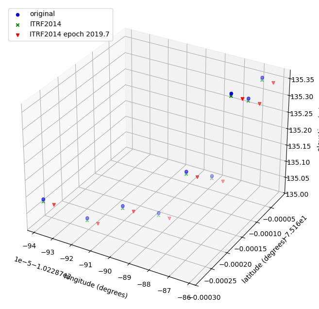
Visualizing the differences
To visualize the differences, which are very small, we need to zoom in on just a small subset of points. First we set a filter condition and apply it to each DataFrame.
filter_condition = (iceflow_df.reset_index().index > 50) & (
    iceflow_df.reset_index().index < 60
)
sampled_iceflow_df = iceflow_df[filter_condition]
sampled_itrf2014_df = itrf2014_df[filter_condition]
sampled_itrf2014_epoch_2019_7_df = itrf2014_epoch_2019_7_df[filter_condition]
Now we create a 3D plot using matplotlib to visualize the differences across latitude, longitude, and elevation.
fig = plt.figure(figsize=(10, 8))
ax = fig.add_subplot(111, projection="3d")
ax.scatter(
    sampled_iceflow_df.longitude.values,
    sampled_iceflow_df.latitude.values,
    sampled_iceflow_df.elevation.values,
    color="blue",
    marker="o",
    label="original",
)

ax.scatter(
    sampled_itrf2014_df.longitude.values,
    sampled_itrf2014_df.latitude.values,
    sampled_itrf2014_df.elevation.values,
    color="green",
    marker="x",
    label="ITRF2014",
)

ax.scatter(
    sampled_itrf2014_epoch_2019_7_df.longitude.values,
    sampled_itrf2014_epoch_2019_7_df.latitude.values,
    sampled_itrf2014_epoch_2019_7_df.elevation.values,
    color="red",
    marker="v",
    label="ITRF2014 epoch 2019.7",
)

ax.set_xlabel("longitude (degrees)", labelpad=10)
ax.set_ylabel("latitude (degrees)", labelpad=10)
ax.set_zlabel("elevation (m)", labelpad=10)
plt.legend(loc="upper left")
plt.show()